By Hélio E. Sueta; Luís E. Caires; Roberto Zilles – Instituto de Energia e Ambiente [Institute of Energy and Environment] (USP)
Content kindly provided for publication on the GRUPO INTELLI website by Hélio E. Sueta, Luís E. Caires, and Roberto Zilles.

Abstract

This paper presents a study for the use of copper clad steel cables in Lightning Protection Systems (LPS).

The main objective of this study is to help define the section of this type of cables for the protection systems.

INTRODUÇÃO

The IEC 62305-3: 2010 [01] standard, as well as the Brazilian standard ABNT NBR 5419-3: 2015 [02] allows the use of copper clad steel cables in lightning protection systems.

The IEC [01] in its Tables 6 (“Material, configuration and minimum cross-sectional area of air-termination conductors, air-termination rods, earth lead-in rods and down-conductors) and 7 (“Material, configuration and minimum dimensions of earth electrodes) indicate a cross-sectional area of 50 mm² for copper coated steel, in “solid round” configuration (earth rod diameter 14 mm, with a note that “in some countries the diameter may be reduced to 12.7 mm ”) as “solid tape” and respectively 50 mm² and 90 mm² in Table 7 which refer to the minimum dimensions of earth electrodes.

In its Table 6 referring to the conductors of the airtermination and down-conductor subsystems, ABNT NBR 5419-3: 2015 [02] indicates a minimum section area of 50 mm² in the configurations “Solid Round” (diameter 8 mm) and “corded” (diameter of each wire of the strand 3 mm) for the 30% IACS copper coated steel cable. In Table 7, that refers to the earth-termination electrode, the values indicated are sections of 70 mm² for the non-spiked electrode (with a diameter of 3.45 mm for each wire of the strand) and a minimum diameter of 12.7 mm for the spiked electrode for the “rounded solid” and “corded” configurations for copper-coated steel.

The differences between the international and the Brazilian standards values in the dimensions of these conductors led to a study to verify the behavior of copper clad steel conductors in their use in Lightning Protection Systems (LPS).

The aim of this paper was to study copper clad steel wire cables compared to copper cables. These are the studied cables characteristics:

• Bare copper cable, sections 35 mm² (7 wires x 2.5 mm) and 50 mm² (7 wires x 3 mm).
• Copper clad steel wire cable, section 35 mm², 30%, 40% and 53% IACS, LCA (7 wires x 2.5 mm) and section 50 mm², 30%, 40% and 53% IACS, LCA (7 wires x 3mm).

Tests were carried out at the Institute of Energy and Environment of the University of São Paulo to simulate the thermal effects on the cables (application of direct current pulses in the form of an electric arc simulating the continuing current component of lightning), short circuit tests (on 60 Hz) and temperature rise tests (also at 60 Hz).

BASIC CONSIDERATIONS

The IACS is a unit of measurement for electrical conductivity which is a microscopic property of materials that corresponds to the inverse of resistivity. This unit of measurement is frequently used in Great Britain and USA.

The specific electrical conductivity of 100% IACS corresponds to 58 MS/m (million Siemens per meter). Conductivity values given in % IACS imply that measurements were taken at a temperature of 20°C (293K or 68°F). Measurements indicated in MS/m need to inform the temperature at which they were taken.

The tests were performed on stranded cables with two different sections: 35 mm² and 50 mm². In the case of copper, this type of cable is used as a conductor for the air-termination and down conductor subsystems with a section of 35 mm², with a diameter of 2.5 mm for each strand wire and in the earth-termination subsystem with a section of 50 mm², with the diameter of each wire of the strand being 3 mm.

DEVELOPMENTS

A structure (see Figure 1) with a length of just over 11 meters (11.2 m) was used where the samples were installed and pulled.

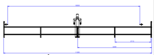
Figure 1 - Experimental set-up for tests

TESTS TO SIMULATE LIGHTNING

In the tests to simulate the continuing current, the specimens were installed and tensioned with 15% of the RMC of the cable, which in the case of the 35 mm² varies from 137 to 177 daN and, in the case of the 50 mm², it varies from 173 to 251 daN.

The direct current pulse to simulate the continuing current component has a charge of approximately 200 Coulombs (pulse of approximately 400 A and application time of 500 ms). This test was performed on three samples of each type.

Figure 2 shows an oscillogram of the direct current pulse applied to one of the samples.

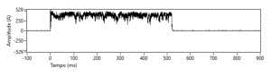
Figure 2 - Current oscillogram of the lightning simulation test

After applying the pulse in the arc form in the center of the length of the sample, the value of the tensile load is verified and recorded for each sample (which is after 3 minutes of application). A visual inspection is made at the point where the arc occurred. After this verification, each specimen is pulled at a load of 40% of the cable's RMC maintained for 3 minutes in that pull.

The tests were based on the ABNT NBR 14074 [03] standard, in Annex B, which is the standard for optical fiber grounding cables (OPGW) for overhead transmission lines – requirements and test methods. This standard was used because it contains the lightning test on cables.

The electrode used is 1020 steel and was installed as shown in Figure 3, where the "gap" between the electrode and the sample was adjusted to 60 mm, with an approximate inclination of 45º in relation to the plane of the sample (parallel to the plane of the sample test bench). Three tests were performed on each type of sample, with one application on each sample.

Table I describes the measured values for each sample with section #35 mm² in the lightning tests. In Table II, for cables of #50 mm². Tables I and II will be presented at the end of this paper, as well as some figures of the cables after the tests.

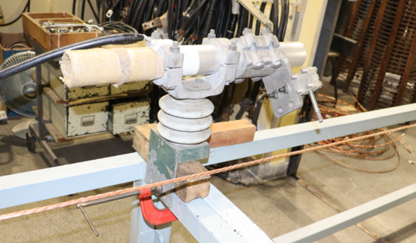
Figure 3 - Electrode layout for the lightning simulation test

SHORT-CIRCUIT TESTS

The tests were carried out with a symmetrical current of 7 kA (effective value) for cables with a 35 mm² section and 10 kA for a 50 mm² section ones, with an application time of 500 ms. It was applied one application in each sample.

The maximum temperature reached in the tests was verified and the mechanical deformations in each sample were analyzed.

Each sample was installed on the structure (Figure 1) and initially pulled at approximately 200 kgf for the #35 mm² section samples and 250 kgf for the #50 mm² section samples.

In each application, the following parameters were measured and recorded: current, voltage between two points at the extremes of the samples, active power and temperature at the central point of the sample. For measuring and recording current, voltage and power, the following system was used:

• Digital oscilloscope (digital scope DL850); manufacturer: YOKOGAWA.
• Current transducers (power unit); manufacturer: YOKOGAWA.

Three methodologies were used to measure the temperature: thermocouple measurement; measurement through a thermal imager and by calculation through the variation of electrical resistance.

In the case of measurements using a thermocouple and a thermal imager, the values were obtained from the direct reading of the instruments. The maximum values indicated by the instruments were recorded.

The equipment used were:

• Digital multimeter, manufacturer: MINIPA, model: ET-2517, Serial number: ET-251700183. Fitted with a “K” type thermocouple.
• Thermal Imager Manufacturer: FLIR, Serial Number: 49003207, Model: E50.

In the case of determining the temperature by calculation through resistance variation, data from the measurement system were used to calculate the instantaneous power. From these values, the active power per cycle was calculated. The effective value of the current per cycle was also calculated. From these values, the resistance per cycle was calculated.

As an auxiliary parameter, a mechanical load (traction) was applied, which was measured by a load cell (manufactured by Oswaldo Filizola, Crown DAC model).

Table III describes the values measured for each sample in the short circuit test. Figure 4 below illustrates the load cell.

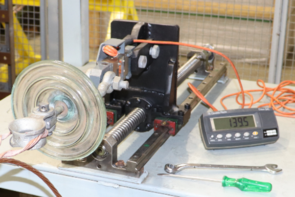
Figure 4 - Mechanical load measurement system (traction)

An example of applying the concept, can be the process used in sample 07, a 50 mm² copper cable. For this, it was necessary to have the value of T0 or α, which are constants related to the resistance variation with temperature. In practice, these values are equivalent, differing only in the application of the concept. There is an expression that establishes this equivalence, which is:

T0+20=1/α

It is not the objective of this paper to discuss the theory involved in this matter, only to indicate the steps followed to obtain the values. Having the value of T0 (which in this case is 234.5°C) it was possible to apply it to the short-circuit test and it was estimated in this case that the temperature reached 181°C by the resistance
variation.

The thermocouple measuring system recorded 150°C and the infrared radiation measuring system recorded 126°C, as shown in Figure 5 below.

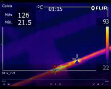
Figure 5 - Example of thermography of one of the samples

The problem is that this value was recorded after the application when the conductor stopped moving after the electromagnetic effort inherent to the short circuit under these conditions. Thus, it is expected that the recorded temperature was lower than the maximum. To get around this difficulty, oscillographic records were used in order
to calculate the temperature as a function of resistance (see Figure 6). The following graphics illustrate the stepby-step process.

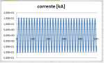
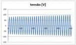
Figure 6 - Short-circuit current and voltage oscillograms The test current (approximately 10kA effective) was applied and the voltage drop across the sample was recorded. With this, the power variation as a function of time was obtained (see Figure7).

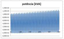
Figure 7 - Power oscillogram in the short-circuit test

The power increases as a result of the increase in resistance of the conductor due to heating. The resistance value can be obtained cycle by cycle by calculating the values of active power and effective current per cycle, thus obtaining a graph of resistance variation as a function of time in steps (Figure 8).

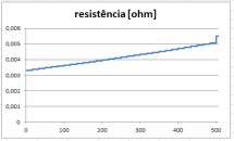
Figure 8 - Resistance variation during the short circuit test

From the resistance values and taking the value of T0, the temperature behavior of the sample was calculated (see Figure 9).

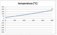
Figure 9 - Temperature variation during the short circuit test

This entire process was carried out for all samples, obtaining the indicated results (Table III).

TEMPERATURE RISE TESTS

The tests were carried out on cables with 53% IACS and with currents, 60 Hz, of 193 A for cables with a  section of 35 mm² and of 242 A for the 50 mm² ones. The cable manufacturer has indicated these values.

The tests were performed on each sample with current conduction until temperature stabilization. Temperatures were measured using suitable thermocouples. Temperatures were recorded at some points in the sample and the ambient one to obtain the temperature rise.

The temperatures reached in the tests were according to table IV below:

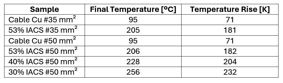
TABLE IV - Temperature rise test

RESULTS AND THEORETICAL DEVELOPMENTS

Both the IEC 62305-1: 2010 [04] standard and the Brazilian standard ABNT NBR 5419-1: 2015 [05] present Tables “D.2 – Physical characteristics of typical materials used in LPS components” and “D.3 – Temperature rise for conductors of different sections as a function of W/R”.

This study, based on the tests carried out, mainly in the short circuit and the temperature rise, completes these tables with parameters for steel cables covered with copper IACS 53%, IACS 40% and IACS 30%, in addition to comparing the results obtained for copper with the tabulated values.

Using equation D.7 described in both IEC 62305: 2010 and ABNT NBR 5419-1: 2015 and the test results, Table D.2.REV. (see at the end of the paper) complements Table D.2 in the standards.

To obtain the parameters for copper-covered steel cables, the following considerations were made:

• Test data and those obtained from the literature were considered, which include the standards [04, 05], aiming to make the models compatible in order to have a comparison parameter.
• Taking the values for copper and mild steel, equivalent resistance values were calculated for the compositions that resulted in conductivities of 53%, 40% and 30% IACS. From these values, the values of resistivity ρ0 and temperature coefficient α were calculated. The values were applied to the normalized expression and compared to the results obtained during the tests in order to validate the parameters. The results of the comparison are listed at the end of the paper, along with table D.3.REV.
• The same variables as in the standard were used to characterize the materials: ρ0 is the specific ohmic resistance of a conductor at ambient temperature, γ is the material density, Cw is the thermal capacity, Cs is the latent heat of fusion and ϴs is the melting temperature.

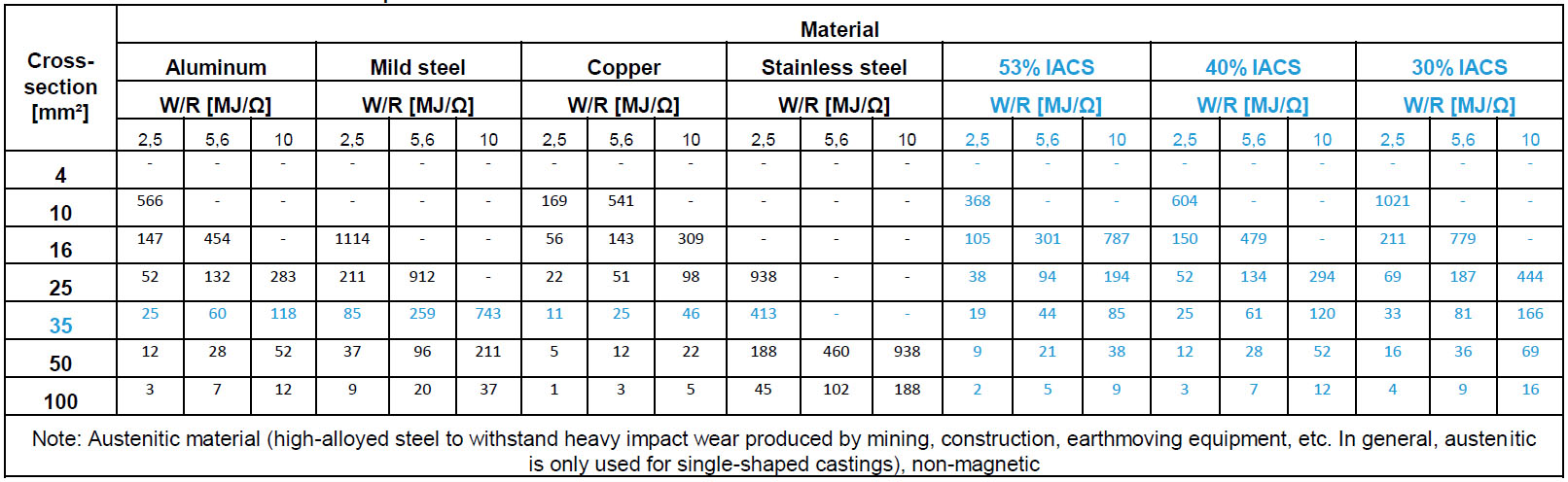
Table D.3 was also revised and complemented with the values for cables with a #35 mm² section, widely used in LPS, and with the values for steel cables covered with copper, creating the new Table D.3.REV ( see at the end of the paper).

In preparing this revised table, the following considerations were made:

The expression of the Brazilian standard ABNT NBR 5419-1: 2015 [05] was used to calculate the temperature rise in the cable as a function of W/R, verifying the compatibility of the results for the existing materials in the standardized table. The other materials not included in the standard table were calculated from the new parameters in table D.2.REV.

Only the values for copper cables 35mm² and 50mm², 30%, 40% and 53% IACS that were tested in the laboratory were compared.

Laboratory applications were made with approximately 50MJ/Ω for 50 mm² cables and 25MJ/Ω for 35 mm² cables. These values are far above the tabulated values so that it was possible to obtain the values for 2.5; 5.6 and 10 MJ/Ω. However, these values were obtained from the analysis of current, voltage and power waves during applications and curve fitting techniques in order to obtain the best approximation. The values obtained were within the range of tested values and no extrapolation was performed.

Thus, it is possible to create a table with values calculated through the expression of the standard, as well as to obtain the corresponding values obtained from the analysis of the test data.

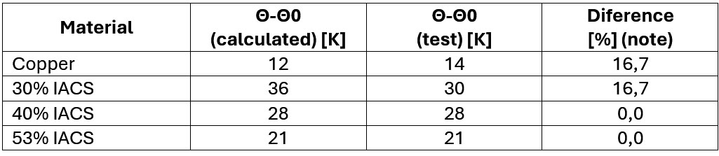
Considering W/R 50 MJ/Ω for a 50 mm² cable.

The values obtained are close, but with a considerable difference due to the difficulty of accurately determining the temperature of the cable. Three methods were used, but each of them has limitations that made it difficult to measure the temperature accurately.

Considering W/R 2.5 MJ/Ω for a 50 mm² cable.

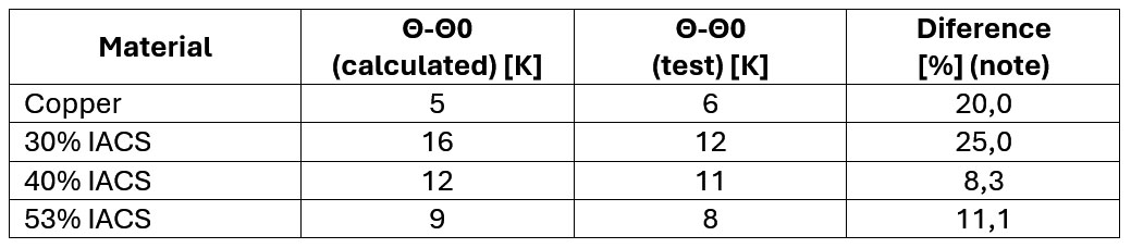
Considering W/R 5.6 MJ/Ω for a 50 mm² cable.

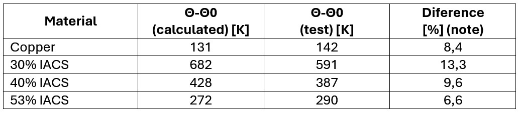
Considering W/R 10 MJ/Ω for a 50 mm² cable.

Note: Module of percentage values in relation to the calculated value.

Comparing the values obtained, it is observed that they are compatible with each other with acceptable differences (around 10% on average) considering the limitations and difficulties inherent to the test. Interestingly, the highest percentage error values correspond to the lowest absolute error values, as they occurred with low temperature rise values, where a difference of only 1 K is percentage more significant.

Combinations of 35 and 50 mm² cables were tested, which resulted in a considerable number of tests, laboratory hours and data for processing and analysis. In addition, the cost of samples cannot be overlooked either.

As can be seen from table D.3.REV, testing all the configurations found therein would add an unnecessary burden to the process without significantly improving accuracy. Thus, the other values in this table were obtained by calculation, since these results must be compatible with the tests within an acceptable margin of error.

ANALYSIS OF THE RESULTS

Short circuit test

The short-circuit tests showed that none of the samples broke (none of the wires that make up the cables), only the colors of some samples changed in relation to the original state.

Temperature measurements in the central span of the samples by different methods showed close results, however with specific measurement problems.

As the samples are approximately 20 meters long each, due to the test setups, the currents involved and the electromagnetic interaction in the loop, mechanical efforts occur, causing the cables to move a lot in the tests. Furthermore, as there was a considerable temperature increase in some samples, the corresponding expansion also influenced the movement of the cables.

This movement, added to the very sudden temperature variation, the high values it reaches and the short test time, lead to difficulties in measuring the maximum temperature at the central point of the samples.

In the case of measurement through thermocouples, the choice of thermocouple type is important, as well as the way of fixing it in the sample. In these tests, a “K” type thermocouple was used, which was fixed in different ways, until a way was chosen that would make it firmer, in order to minimize the deterioration of its insulation and of the means of fixation due to the high reached temperature values. The temperature-measuring device must also have a good response time with the ability to record at least the maximum value reached.

The digital multimeter, manufacturer: MINIPA, model: ET-2517, was used in the test, which shows the current temperature and records the minimum and maximum values.

When measuring using the thermal imager, special care must be taken in relation to the temperature limit of the device and the emissivity adjustment of the point to be measured. In this test, in particular, check whether the area covered by the measurement will contain the scattering due to the movement of the cable during the short circuit.
The calculation of the temperature through the variation of the electrical resistance proved to be quite reasonable. During the short-circuit tests, the test current, the voltage between two points of the sample and the active power and effective value of the current per cycle were recorded. With these values it was possible to analyze the data to obtain and follow the variation of the electrical resistance of the sample and through this to calculate the temperature of the cable.

For cables with a section #35 mm², the initial traction applied to the samples was approximately 200 kgf and for those with a section #50 mm² it was 250 kgf.

During the applications of the short circuit, a great elongation in the length of the samples was verified, which was reduced until reaching approximately the initial length as the samples cooled close to the ambient temperature. Measurements of the length of the samples were not made before and after the applications in these tests, but it is assumed that there was considerable expansion of the cables.

As expected, the maximum temperatures obtained in the copper-covered steel cables were significantly higher than those reached by the copper cable were. The IACS 53% samples showed lower temperatures than the other IACS, but still above those of the copper cables. After the short-circuit applications, a change in the color of the samples was observed, especially in those with higher temperatures.

Lightning simulation test

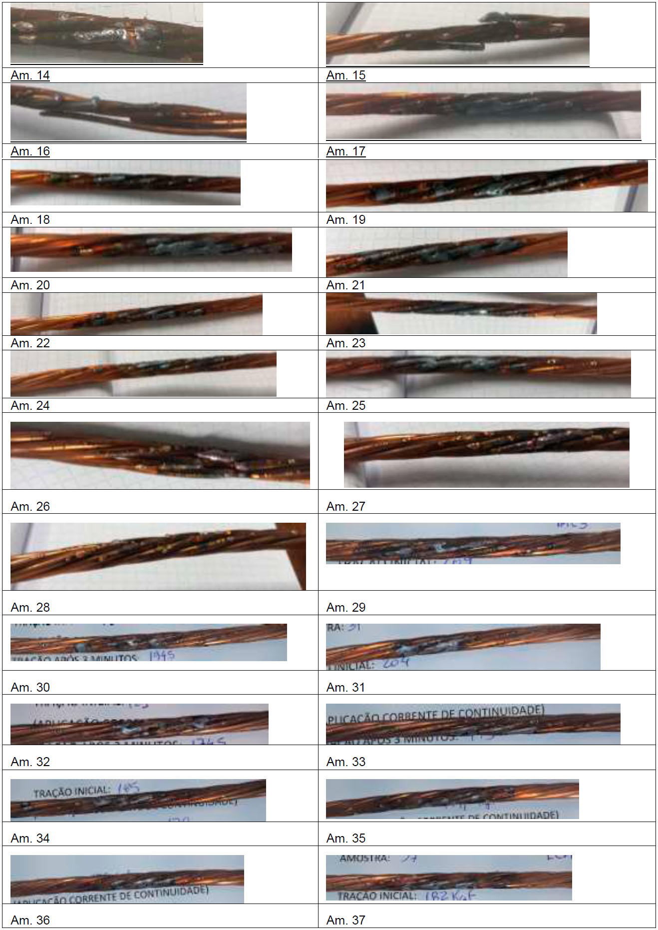
In the lightning simulation test, the direct current pulse was applied in the form of an electric arc. Unlike the samples with copper cable, where wire breakages (one or two wires) were observed during the applications, the samples with copper-covered steel cable did not have any broken wires. Visual damage is observed (see Photos), but all samples withstood increased tension to 40% of cable RMC for 3 minutes after lightning tests.

Temperature rise test

In the temperature rise tests, the temperature stabilized at the values indicated in item 3.3 (Table IV).

This test was used to guide the estimates of temperature rise in the cables in the short-circuit tests, since in this case it is possible to follow the resistance and temperature variation by thermocouple, under stable and controlled conditions for the use of these elements measurement.

The following graph (Figure 10) for a 50 mm² 40% IACS cable sample demonstrates the behavior of the temperature values estimated by the resistance variation method (in blue) and those recorded by the system that used thermocouple (in red).

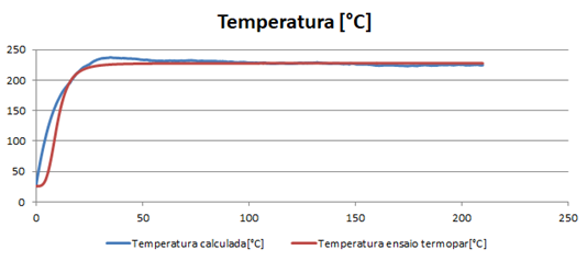
Figure 10 - Graphs of temperatures recorded in the elevation test

Tests carried out on all tested samples showed similar graphs both for the resistance variation method and for the records obtained from the thermocouple measurement system.

Study of material parameters

Both in IEC 62305 and in ABNT NBR 5419, the parameters for copper-covered steel cables (IACS 52%, IACS 40% and IACS30%) do not appear, neither in Table D.2 nor in Table D.3. This study presents these values with reasonable reliability, since the others already tabulated were confirmed by the same procedure, which included laboratory tests.

Although the parameters for these materials are not included in the standard tables, through the study of existing values, catalog and literature data and the use of relatively simple analysis methods accompanied by laboratory tests, it was possible to deduce the elements that complete the normalized tables.

The virtue of using the standard as a reference was to aggregate the body of data collected during the test into a set of information organized according to an already known and well-founded criterion. Translating the test data into standards-compliant format was straightforward, as the measured parameters made it easy.

CONCLUSIONS

This paper presents a study on copper clad steel cables with the objective of helping to normalize the section of these cables for use in lightning protection systems.

The study is based on tests in laboratories focusing on some sections and types of cables with different electrical conductivity.

Copper clad steel cables can be used as a component of the LPS and the sections described in Tables 6 and 7 of ABNT NBR 5419-3: 2015 must be reviewed, and may be, in Table 6 referring to the conductors used in the air-termination system and of down-conductors system, a minimum section area for copper-plated steel and a minimum conductivity of 30% IACS, of 35 mm² and for Table 7 which refers to conductors for the earth-termination system, a minimum section, for non-crimped electrodes, of 50 mm². When using these types of copper-plated steel cables in contact with other materials that may be combustible, the physical characteristics of these materials and the temperature rises described in Tables D.2.REV and D.3.REV, described in this report, must be considered.

The use of these copper clad steel cables in other systems, for example, as grounding cables for substation electrical installations or for power cables, must be studied on a case-by-case basis, taking into account the results and characteristics of the tests carried out, mainly short-circuit and temperature rise tests.

Anexes

TABLE I - Parameters used in each lightning test application - #35 mm² section cables

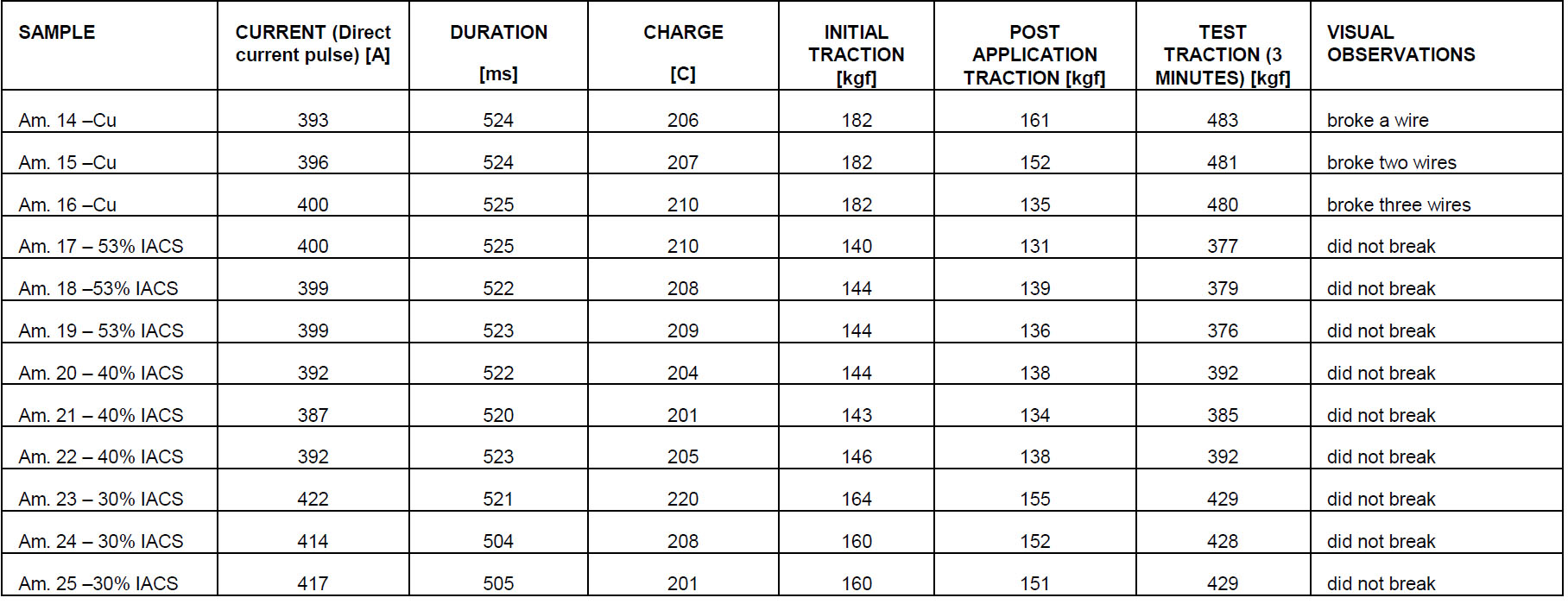
TABLE II - Parameters used in each lightning test application - #50 mm² section cables

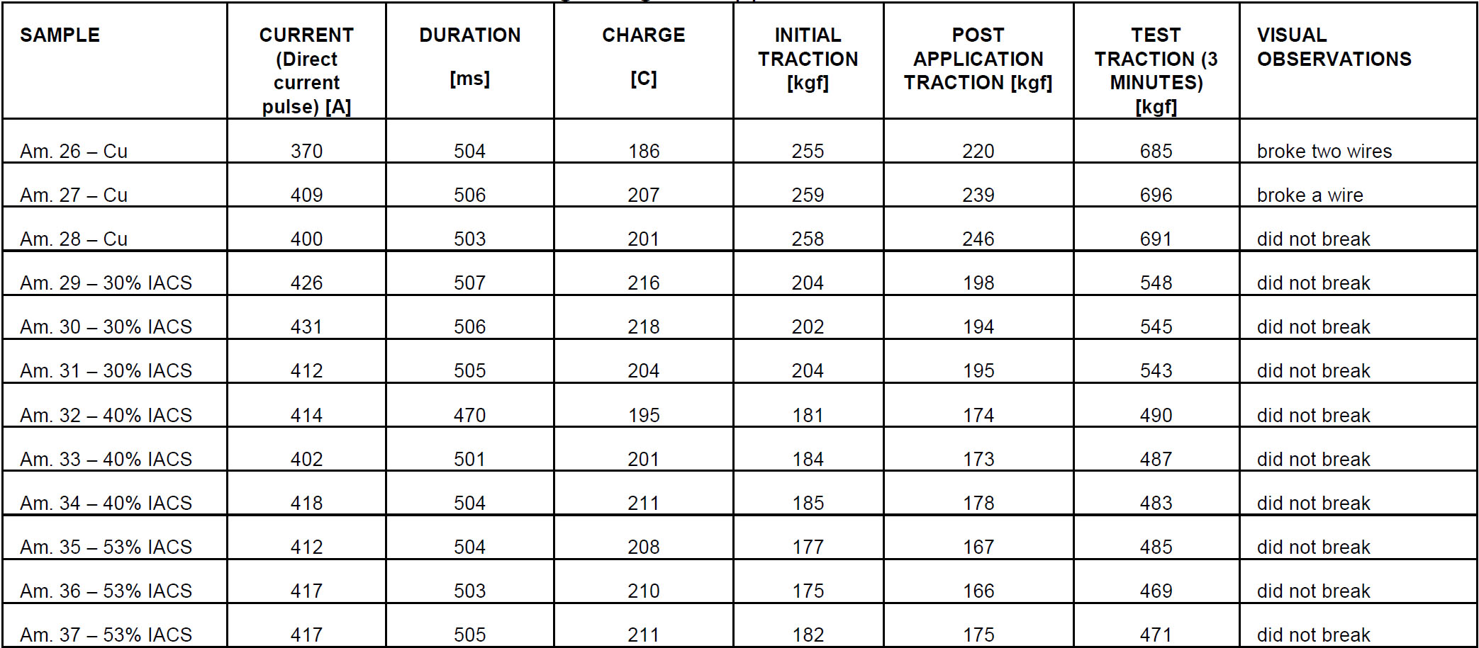
TABLE III - Parameters used in each short circuit test application

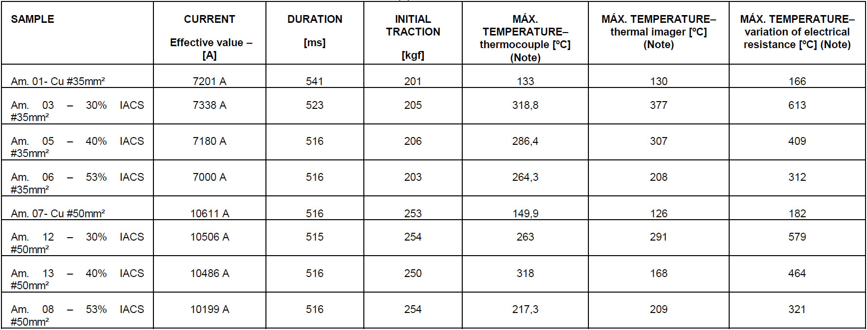
Note: Maximum thermocouple and thermal imager temperatures were obtained by direct reading. The temperatures obtained by the resistance variation were calculated and represent the central (mean) value of the range of estimated values for the maximum temperature value.

Table D.2.REV – Physical characteristics of typical materials used in revised LPS components.

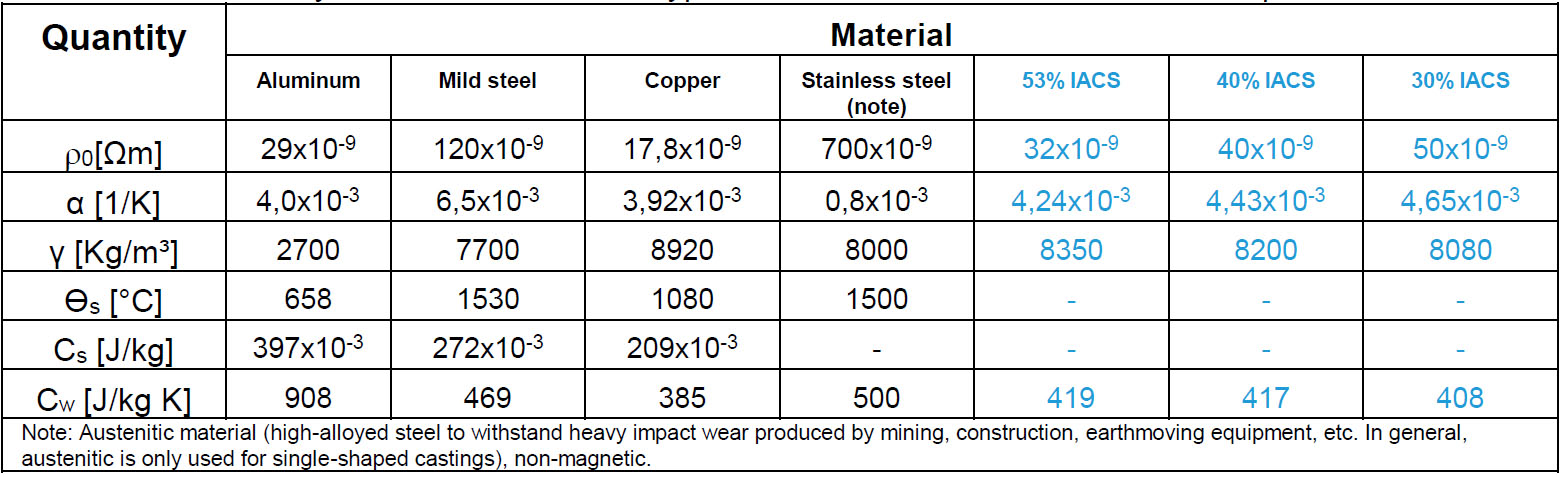
Table D.3.REV – Temperature rise for conductors of different sections as a function of revised W/R.

PHOTOS AFTER LIGHTNING TESTS

REFERENCES

[1] IEC – INTERNATIONAL ELECTROTECHNICAL COMMISSION, “IEC 62305-3: 2010 – Protection against lightning – Part 3: Physical damage to structures and life hazard”, 2010.

[2] ABNT – Associação Brasileira de Normas Técnicas, “ABNT NBR 5419-3: 2015 – Proteção contra descargas atmosféricas – Parte 3: Danos físicos a estruturas e perigos à vida”, 2015, in portuguese.

[3] ABNT – Associação Brasileira de Normas Técnicas, “ABNT NBR 14074: 2015 - Cabos para-raios com fibras ópticas (OPGW) para linhas aéreas de transmissão – Requisitos e Métodos de ensaio”, 2015, in portuguese.

[4] IEC – INTERNATIONAL ELECTROTECHNICAL COMMISSION, “IEC 62305-1: 2010 – Protection against lightning – Part 1: General Principles”, 2010.

[5] ABNT – Associação Brasileira de Normas Técnicas, “ABNT NBR 5419-1: 2015 – Proteção contra descargas atmosféricas – Parte 1: Princípios Gerais”, 2015.